Glossary – Data Analytics

• Selection bias: Occurs when the subjects in a study are not chosen at random, leading to a non-representative sample.
• Measurement bias: Occurs when the instruments or methods used to collect data are not valid or reliable.
• Confounding bias: Occurs when an extraneous variable is not controlled for and affects the relationship between the independent and dependent variables.
• Publication bias: Occurs when studies with significant or positive results are more likely to be published or reported than studies with non-significant or negative results.

It is important to be aware of potential sources of bias in a study and to take steps to minimize or control for them, in order to ensure the validity and reliability of the results.

• Unstructured Correlation:This assumes that all pairwise correlations between observations are distinct and unrelated to one another. Unstructured correlation is often used with linear regression models.
• First-Order Autoregressive Correlation: This assumes that observations that are closer in time are more strongly correlated than observations that are further apart. First-order autoregressive correlation is often used in time series models and repeated measures analyses.
• Exchangeable Correlation: This assumes that all observations are equally correlated with one another. Exchangeable correlation is often used in multilevel models with a random intercept.
• Compound Symmetry Correlation: This assumes that all pairwise correlations are the same and that observations are equally correlated with one another. Compound symmetry correlation is often used in multilevel models with a random intercept.
• Toeplitz Correlation: This assumes that the correlation between observations decreases as the distance between them increases. Toeplitz correlation is often used in time series models and repeated measures analyses.
• Block Correlation: This assumes that observations within the same block are more strongly correlated with one another than with observations in other blocks. Block correlation is often used in clustered data or repeated measures analyses.

• Organic data sets: These are data sets that are naturally occurring and are collected in the course of normal business or research activities. For example, a retail store might collect data on sales transactions, a hospital might collect data on patient visits, and a university might collect data on student enrollment. These data sets are often unstructured and may contain missing or inconsistent data.
• Designed data sets: These are data sets that are specifically created for a research or other specific purpose. For example, a researcher might conduct a survey and collect data on a specific topic, a company might conduct an experiment to test a new product, or a government agency might collect data on crime rates in a specific area. These data sets are often structured, with a specific set of variables and a specific format for collecting and reporting the data.

Both types of data sets are important for research and analysis. Organic data sets provide a natural context and can be used to understand real-world phenomena, while designed data sets allow for more controlled and precise research.

It’s worth noting that there is also a third type of data sets, synthetic data sets which are artificially created data sets, to be used for specific purposes such as testing, training, or creating a proxy of real-world data when it is not possible to have access to the real data.

The key feature of GEE is that it provides population-average or marginal estimates of the regression coefficients, which reflect the average effect of the predictor variables on the outcome variable across all subjects, regardless of the correlation structure. This is in contrast to the subject-specific or conditional estimates provided by other methods such as mixed-effects models.

GEE can handle a wide range of outcome variables, including binary, count, and continuous outcomes, and can accommodate a variety of correlation structures, such as exchangeable, autoregressive, and unstructured. GEE is also robust to misspecification of the correlation structure and can be used with missing data.

GEE is used in a variety of settings, including longitudinal studies, cluster-randomized trials, and repeated measures designs. It is particularly useful when the focus is on the population average effect of predictor variables rather than the subject-specific effect. It is also useful when the correlation structure is unknown or difficult to model accurately.

Overall, GEE is a flexible and widely used approach for analyzing correlated data, and it has become an important tool in statistical analysis of longitudinal and clustered data.

• Independent: The data points or observations are considered independent if the value of one observation does not depend on the value of any other observation. This means that the probability of any given outcome does not change based on the values of any other outcome.
• Identically Distributed: The data points or observations are considered identically distributed if they are all drawn from the same underlying probability distribution. This means that the probability of any given outcome is the same for all observations.

Together, these assumptions mean that the data points or observations in a dataset are independent of one another and have the same probability distribution. This is important because it allows for the use of certain statistical techniques and models, such as the central limit theorem, which is the foundation for many commonly used statistical methods, such as t-test, ANOVA, and linear regression.

It’s important to note that these assumptions are not always met in real-world data. However, in many cases, assuming i.i.d. simplifies the analysis and yields results that are approximately correct.

• Mean (arithmetic average):The sum of all the data points divided by the number of data points. It is the most commonly used measure of central tendency. It is sensitive to outliers and extreme values.
• Median: The middle value of a set of data when it is arranged in numerical order. It is the value that separates the data into two equal parts: half of the data is above the median, and half is below. It is a more robust measure of central tendency than the mean and it is not affected by outliers and extreme values.

• Start with a known list (sampling frame) of N population units, and select n units from the list.
• Probabilities cannot be determined for sampled units.
• No random selection of individual units.
• Sample can be divided into groups (strata) or clusters, but the clusters are not randomly sampled in an earlier stage.
• Data collection often very cheap relative to probability sampling.

• Start with a known list (sampling frame) of N population units, and randomly select n units from the list.
• Every unit has equal probability of selection = n/N.
• All possible samples of size n are equally likely.
• Estimates of means, proportions, and totals based on SRS are unbiased (equal to the population values on average).

Sampling can performed with replacement or without replacement: for both the probability of selection for each unit is still n/N.

Types of probability sampling include:

• Simple random sampling (SRS): Every single unit in the sample has the same known probability of being selected. This is the closest probability sampling analog to i.i.d., in that the sampling mechanism used to generate the observations will produce independent and identically distributed observations. SRS is rarely used in practice. Collecting data from n randomly sample units in a large population can be prohibitively expensive, especially if the units at widely dispersed geographically or otherwise difficult to access.
• Complex sampling: Units in the sample have a known probability of being selected, but the probability of various units will differ based on a defined multi-layer sampling methodology(strata, clusters, various levels of sub-clusters, and units within the lowest level sub-clusters). A a unit’s probability of selection is determined by:
  • Number of strata within the total sample population;
  • Number of strata sampled from the total sample population;
  • Total number of clusters within each stratum;
  • Number of clusters sampled from within each stratum;
  • Total number on sub-clusters in each cluster and sub-cluster;
  • Number of units ultimately sampled from each sub-cluster;
  • Total number of units in each ultimate sub-cluster.

• Python Programs for Data Analysis: There are several important Python libraries for data analysis, including:
  • NumPy (Numerical Python): A library for the Python programming language, adding support for large, multi-dimensional arrays and matrices, along with a large collection of high-level mathematical functions to operate on these arrays. It is often used as a fundamental library for scientific computing and data analysis. https://numpy.org/
  • Pandas: A library for data manipulation and analysis. It provides data structures and operations for manipulating numerical tables and time series data. It is widely used for data cleaning and preparation, and is also very useful for data exploration and analysis.https://pandas.pydata.org/
  • SciPy (Scientific Python): A library for scientific and technical computing in Python. It is built on top of NumPy and provides additional functionality for optimization, signal processing, statistics, and more. https://scipy.org/

  

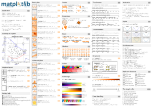
  • Matplotlib: A plotting library for the Python programming language and its numerical mathematics extension NumPy. It provides an object-oriented API for embedding plots into applications using general-purpose GUI toolkits like Tkinter, wxPython, Qt, or GTK. https://matplotlib.org/
  • Seaborn: A data visualization library for Python. It is built on top of Matplotlib and provides a high-level interface for creating attractive and informative statistical graphics. It is particularly well-suited for visualizing complex datasets with multiple variables.https://seaborn.pydata.org/
  • Scikit-learn (also known as sklearn): A library for machine learning in Python. It provides a range of tools for model selection, evaluation, and preprocessing, as well as a variety of commonly used machine learning algorithms such as linear and logistic regression, decision trees, and k-means clustering.https://scikit-learn.org/stable/
  • Statsmodels: A library for estimating and analyzing statistical models in Python. It provides a range of tools for fitting models, estimating parameters, and performing hypothesis tests. It is particularly useful for linear and generalized linear models, as well as time series analysis.https://www.statsmodels.org/stable/index.html
  • Keras and Tensorflow: Keras is a deep learning library for Python, while TensorFlow is a library for numerical computation that allows to create and execute computations that involve tensors. These libraries provide a high-level interface for building and training neural networks, which are widely used for image, text and audio processing, among other things.https://keras.io/ https://www.tensorflow.org/

  These are some of the most popular libraries for data analysis in Python, but there are many others available depending on the specific needs of the project.

• MATLIB is a programming language and software environment for scientific computing, engineering, and data analysis. It provides a wide range of tools for data analysis, including statistical methods, machine learning, and signal processing. MATLAB is widely used in academia and industry for scientific computing and data analysis
• R is a free and open-source programming language and software environment for statistical computing and graphics. It provides a wide range of statistical and graphical techniques, including linear and nonlinear modeling, classical statistical tests, time-series analysis, clustering, and more. R is highly extensible and has a large community of users and developers, with many packages and libraries available for various statistical methods and applications.
• SAS is a software suite for advanced analytics, data management, and business intelligence. It provides a wide range of statistical and data analysis methods, including regression analysis, time-series analysis, data mining, and more. SAS is widely used in industry and academia, and provides a comprehensive set of tools for data analysis and reporting.
• SPSS (Statistical Package for the Social Sciences) is a software package for statistical analysis and data management. It provides a wide range of statistical and graphical techniques, including descriptive statistics, correlation analysis, regression analysis, and more. SPSS is widely used in the social sciences, market research, and other fields where data analysis is important.
• STAN is a a state-of-the-art platform for statistical modeling and high-performance statistical computation. Users rely on Stan for statistical modeling, data analysis, and prediction in the social, biological, and physical sciences, engineering, and business.

  Users specify log density functions in Stan’s probabilistic programming language and get:

  • full Bayesian statistical inference with MCMC sampling (NUTS, HMC)
  • approximate Bayesian inference with variational inference (ADVI)
  • penalized maximum likelihood estimation with optimization (L-BFGS)

  Stan’s math library provides differentiable probability functions & linear algebra (C++ autodiff). Additional R packages provide expression-based linear modeling, posterior visualization, and leave-one-out cross-validation.https://mc-stan.org/

• Stata is a statistical software package that provides a wide range of statistical methods for data analysis and modeling. It includes features such as data management, graphics, and a programming language. Stata is widely used in the social sciences, economics, and other fields where data analysis is important.

Each of these software languages and services has its own strengths and weaknesses, and the choice of which to use depends on the specific needs and preferences of the user. Many statisticians and data analysts use a combination of these tools, depending on the specific tasks and analyses they need to perform.

• Formulating research questions or hypotheses: This step involves identifying the problem or issue to be studied, and developing research questions or hypotheses that will be addressed by the study.
• Sampling: This step involves selecting a sample of subjects from the population of interest, in order to make inferences about the population based on the sample data.
• Data collection: This step involves using appropriate methods and instruments to collect data from the subjects in the sample.
• Data analysis: This step involves using statistical methods to analyze the data and draw conclusions about the research questions or hypotheses.
• Reporting results: This step involves communicating the results of the study in the form of a research report or publication.

The goal of research studies is to generate new knowledge or understanding about a certain topic or issue, and to make valid and reliable inferences about the population of interest based on the sample data.

Categories of research studies include:

• Confirmatory Versus Exploratory:
  • Confirmatory: Designed to test hypotheses that have been previously formulated, usually based on existing theories or literature. The goal is to provide support or refutation of these hypotheses. Confirmatory studies typically use statistical methods to test the significance of the relationships or differences found between variables.
  • Exploratory: Designed to gain a preliminary understanding of a topic or issue, and to generate new hypotheses or ideas. The goal is to identify patterns, relationships, or themes in the data, rather than to test specific hypotheses. Exploratory studies typically use qualitative methods such as open-ended interviews or observation.
• Comparative Versus Non-Comparative:
  • Comparative: Designed to compare two or more groups of subjects, in order to identify similarities and differences between them. The goal is to assess the impact of an intervention or treatment on a certain outcome, or to compare the effectiveness of different treatments. Comparative studies can be experimental or observational.
  • Non-comparative: Designed to study a single group of subjects, without comparing them to any other group. The goal is to understand the characteristics or experiences of the subjects in isolation. Non-comparative studies can be experimental or observational.
• Observational Versus Experimental:
  • Observational: Designed to observe and record the behavior or characteristics of subjects, without manipulating or controlling any aspect of the study. The goal is to understand the natural relationships or patterns that exist between variables. Observational studies can be comparative or non-comparative.
  • Experimental: Designed to manipulate or control one or more aspects of the study in order to assess their impact on a certain outcome. The goal is to determine cause-and-effect relationships between variables. Experimental studies can be comparative or non-comparative.

• Frequentist Approach is based on the idea that the probability of an event is the long-run frequency of that event occurring in repeated independent trials. In other words, frequentists view probability as objective and measurable, and they estimate population parameters using sample statistics. Frequentist methods involve testing hypotheses and making inferences based on the sample data, and they typically involve the calculation of p-values and confidence intervals. Frequentist methods assume that the data are random samples from a population, and that the population parameters are fixed but unknown.
• Bayesian Approach is based on the idea that probability is a measure of subjective belief, and that we can update our beliefs in light of new evidence using Bayes’ theorem. In other words, Bayesian statisticians view probability as a degree of belief, and they estimate population parameters by combining prior information with sample data. Bayesian methods involve specifying a prior distribution for the population parameters, and then updating this distribution based on the sample data to obtain a posterior distribution. Bayesian methods assume that the population parameters are random variables with their own distribution, and that the data are fixed.

The main difference between the two approaches is in how they treat probability and population parameters. Frequentists view probability as an objective measure of the frequency of events, and they estimate population parameters using sample statistics. Bayesian statisticians view probability as a subjective measure of belief, and they estimate population parameters by combining prior information with sample data.

There are other approaches to statistics, such as likelihood-based methods and non-parametric methods. Likelihood-based methods involve maximizing the likelihood function to estimate the population parameters, while non-parametric methods make fewer assumptions about the underlying distribution of the data and instead rely on distribution-free methods. These approaches can be seen as a middle ground between the frequentist and Bayesian approaches, incorporating some aspects of both.

• Normal distribution (also known as the Gaussian distribution or the bell curve): This is a continuous probability distribution that is symmetric about the mean, with a bell-shaped probability density function. It is commonly used to model a wide range of natural phenomena, such as the distribution of human heights or IQ scores.
• Poisson distribution: This is a discrete probability distribution that describes the number of events that occur in a fixed interval of time or space. It is commonly used to model the number of customers arriving at a store, the number of phone calls received by a call center, or the number of accidents on a stretch of highway.
• Binomial distribution: This is a discrete probability distribution that describes the number of successes in a fixed number of trials. It is commonly used to model the probability of success in a Bernoulli trial, such as the probability of heads in a coin flip.
• Exponential distribution: This is a continuous probability distribution that describes the time between independent events that occur at a constant average rate. It is commonly used to model the time between arrivals of customers to a store, or the time between failures of a machine.
• Uniform distribution: This is a continuous probability distribution where all outcomes are equally likely over a specified interval. It is commonly used in simulations or modeling situations where the outcome is unknown or random.
• Gamma distribution: This is a continuous probability distribution often used to model continuous, non-negative data such as time-to-event data, positive continuous variables, and waiting times.
• Chi-squared distribution: The chi-squared distribution is a distribution of the sum of squares of independent standard normal variables. It is often used in hypothesis testing and in the construction of confidence intervals.
• t-distribution: The t-distribution is a family of distributions that is similar to the normal distribution but has heavier tails. It is used in hypothesis testing and estimation when the sample size is small or the population standard deviation is unknown.
• F-distribution: The F-distribution is a family of distributions that is used in analysis of variance (ANOVA) to test whether two or more population variances are equal.

• Linear Regression is used to analyze the linear relationship between a continuous outcome variable and one or more predictor variables. The goal of linear regression is to estimate the coefficients of the predictor variables that best explain the variability in the outcome variable. The outcome variable is assumed to be continuous and normally distributed, and the relationship between the outcome and predictor variables is assumed to be linear. Linear regression is commonly used in fields such as economics, social sciences, and health research to investigate relationships between variables, make predictions, and identify risk factors for various health outcomes.
• Logistic Regression is used to analyze the relationship between a binary outcome variable and one or more predictor variables. The goal of logistic regression is to estimate the probability of the binary outcome, given the predictor variables. The outcome variable is binary and is typically represented as 0 or 1, and the relationship between the outcome and predictor variables is modeled using a logistic function. Logistic regression is commonly used in fields such as epidemiology, public health, and social sciences to investigate the risk factors for various diseases and outcomes.
• Multilevel Linear Regression is used to analyze data with a hierarchical or clustered structure, where observations are nested within different levels, such as individuals nested within neighborhoods or schools. In multilevel linear regression, the outcome variable is continuous, and the model includes both fixed effects for the predictor variables and random effects for the population variables. The goal of multilevel linear regression is to estimate the effects of the predictor variables at each level, while accounting for the correlation among the observations within the same cluster. Multilevel linear regression is commonly used in fields such as education research, public health, and social sciences to investigate the impact of contextual factors on individual outcomes. Multilevel models are also known as 1) hierarchical linear models, 2) linear mixed-effect models, 3) mixed models, 4) nested data models, 5) random coefficient models, 6) varying coefficient models, 7) random-effects models, 8) random parameter models, 9) split-plot designs, or 10) subject-specific models.
• Multilevel Logistic Regression is used to analyze data with a hierarchical or clustered structure, where observations are nested within different levels, such as individuals nested within neighborhoods or schools. In multilevel logistic regression, the outcome variable is binary, and the model includes both fixed effects for the predictor variables and random effects for the population variables. The goal of multilevel logistic regression is to estimate the effects of the predictor variables at each level, while accounting for the correlation among the observations within the same cluster. Multilevel logistic regression is commonly used in fields such as epidemiology, public health, and social sciences to investigate the effects of contextual factors on binary outcomes.
• Marginal Linear Models Fitted using GEE (Generalized Estimating Equations) are used to analyze correlated data, where observations are not independent. Marginal models provide population-average estimates of the effects of predictor variables on an outcome variable, rather than subject-specific estimates. Marginal linear models are used when the outcome variable is continuous, and marginal logistic models are used when the outcome variable is binary. Marginal models are commonly used in longitudinal studies, cluster-randomized trials, and repeated measures designs to investigate the relationship between predictor variables and outcomes while accounting for the correlation among observations. Marginal models are robust to misspecification of the correlation structure and can handle a variety of correlation structures.
• Marginal Logistic Models Fitted using GEE are used to analyze correlated data with binary outcomes, where observations are not independent. They provide population-averaged estimates of the effects of predictor variables on a binary outcome variable. Like the marginal linear model, the marginal logistic model is fitted using GEE, which allows for a flexible specification of the correlation structure among observations. A marginal logistic model is commonly used in longitudinal studies, cluster-randomized trials, and repeated measures designs to investigate the relationship between predictor variables and outcomes while accounting for the correlation among observations. The marginal logistic model is robust to misspecification of the correlation structure and can handle a variety of correlation structures.
• Time Series Models are used to analyze data that is collected over time, such as stock prices, weather data, or economic indicators. Time series models can be used to forecast future values based on historical data.
• Survival Analysis Models are used to analyze time-to-event data, such as the time until a patient dies or the time until a machine fails. These models can be used to estimate the probability of an event occurring at a certain time, and to identify factors that influence the risk of an event occurring.
• Mixed Effects Models are used to analyze data with both fixed and random effects, such as data from a study with repeated measurements on the same individuals or data from a cluster-randomized trial. These models can be used to estimate the effects of predictor variables on an outcome variable, while accounting for the correlation among observations.
• Bayesian Models are used to estimate the probability of an event occurring, based on prior knowledge or beliefs about the event. Bayesian models can be used to estimate parameters in complex models, and to make predictions based on those estimates.
• Latent Variable Models are used to analyze data with unobserved variables or constructs, such as attitudes, beliefs, or personality traits. These models can be used to estimate the relationships between observed variables and latent variables, and to identify the underlying factors that influence the observed variables.
• Structural Equation Models are used to analyze data with multiple interrelated variables and to test complex hypotheses about the relationships among those variables. These models can be used to estimate the direct and indirect effects of variables on an outcome variable, and to identify the underlying causal relationships among variables.
• HLM (Hierarchical Linear Modeling) is a statistical method used for analyzing data that has a hierarchical structure, such as individuals within groups, students within classrooms, or patients within hospitals. HLM is a type of multilevel modeling, which takes into account the fact that the observations within each group are not independent, and that the groups themselves may differ in terms of their characteristics or effects on the outcome of interest.

  HLM is used to estimate the effects of predictors on an outcome variable, while accounting for the correlation between observations within each group and the variability across groups. The model allows for the estimation of both fixed effects, which are the effects of the predictors on the outcome that are consistent across all groups, and random effects, which are the effects that vary across groups.

  HLM can be used in a wide range of fields, including education, psychology, sociology, and public health. It is often used to study the effects of interventions or treatments on outcomes, such as the effects of different teaching methods on student achievement, or the effects of different healthcare interventions on patient outcomes. HLM can also be used to study the relationship between individual and contextual factors, such as the effects of neighborhood characteristics on health outcomes.

• Polynomial regression is used when the relationship between the outcome variable and one or more predictor variables is not linear. In polynomial regression, a higher-order polynomial function (e.g., quadratic, cubic) is used to model the relationship between the outcome variable and the predictor variables.
• Ridge regression is used when there is multicollinearity among the predictor variables. Ridge regression adds a penalty term to the regression equation to shrink the coefficients of the predictor variables, reducing the impact of multicollinearity and improving the stability of the regression estimates.
• Lasso regression is similar to ridge regression, lasso regression is also used when there is multicollinearity among the predictor variables. However, instead of adding a penalty term to the regression equation, lasso regression uses a penalty term that forces some of the coefficients to be exactly zero, effectively selecting a subset of the most important predictor variables.
• Poisson regression is used when the outcome variable is a count variable and follows a Poisson distribution (e.g., number of accidents in a day, number of hospital visits in a week). Poisson regression models the relationship between the count outcome variable and one or more predictor variables, and provides estimates of the rate of the count outcome as a function of the predictor variables.
• Quantile regression is used when the relationship between the outcome variable and predictor variables may vary across different quantiles of the outcome variable. Quantile regression provides estimates of the effects of predictor variables on different quantiles of the outcome variable, allowing for a more nuanced understanding of the relationship between the predictor variables and the outcome variable.

• Categorical variables can be divided into groups or categories. These variables can be further divided as follows:
  • Ordinal variables have a natural ordering or ranking (e.g, credit grade).
  • Nominal variables do not have a natural ordering or ranking (e.g., property type).

  Binary variables have only two categories or levels. The two levels of a binary variable are typically represented by 0 and 1, or by two labels such as “yes” and “no”, “success” and “failure”, or “male” and “female”.

• Quantitative variables> can be measured numerically. These variables can be further divided as follows:
  • Continuous variables can take on any value within a certain range (e.g., interest rate).
  • Discrete variables can only take on certain specific values (e.g., FICO score).